Introduction
As data scientists we often have a set of observed data and want to “describe” the underlying distribution from which it was generated. The act of describing this distribution is known as fitting the distribution to the data.
Maximum likelihood estimation (MLE) is one such method of distribution fitting in which we consider the likelihood of our data under the proposed distribution and tune the distribution parameters to maximize this likelihood. In this way we find the parameters that yield the highest probability of generating our given sample restricted to the given form of distribution. Let’s make this more concrete.
The Likelihood Function
What do we mean by the likelihood of our data? Well, first assume that our data is a single sample \(X_1\) which comes from some probability distribution.
Then the probability that we get a sample \(x\) is simply \(P(X_1 = x)\). Now assume we have a series of \(n\) independent samples \(X_1, \dots, X_n\) from the same distribution. Then we can use the fact that independence implies our probabilities multiplies to get,
\[P(X_1=x_1, ..., X_n=x_n) = P(X_1=x_1)*\dots*P(X_n=x_n)\]Often times we can characterize a probability distribution with one or several parameters. A parameter is a characteristic of a distribution that defines its behavior and probabilities. Some examples include the width of a uniform distribution or the mean and standard deviation of a normal distribution.
Suppose that our distribution has a single parameter \(\theta\). Then the probability above will be different for different values of \(\theta\). Given that this is the case, we can write down the probability of our sample for a specific value of \(\theta\) with the conditional probability:
\[P(X_1=x_1, \dots X_n=x_n \mid \theta) = \prod_{i=1}^n P(X_i=x_i \mid \theta)\]This is our likelihood function, denoted \(\mathcal{L}(\theta \mid X_1, \dots X_n)\) and it represents how likely our data is under the given value of the parameter theta.
A natural way to fit our distribution to our data is to maximize the likelihood of our data. Intuitively we are saying we have some data that we suspect comes from a given distribution and our best bet is to choose the form of that distribution such that it yields values close to what we sampled.
How do we do this? Note that \(\mathcal{L}(\theta \mid X_1, \dots X_n)\) is a function of \(\theta\). This means we can optimize it via calculus or other means and reach the MLE for the given distribution. While this seems abstract, it can be helpful to apply the method to some example distributions.
Example 1: Poisson Distribution
The poisson distribution has probability distribution function:
\[P(X=k) = \frac{\lambda^k e^{-\lambda}}{k!}\]Then the likelihood function is,
\[\mathcal{L}(\lambda \mid X_1, \dots X_n) = \prod_{i=1}^n \frac{\lambda^{x_i} e^{-\lambda}}{x_i!}\]How do we maximize the value? It is often easier to maximize the log-likelihood and this will yield the same result as the log is monotonically increasing.
The log likelihood in this case is:
\[\begin{align} l(\lambda \mid X_1, \dots , X_n) &= \log{\prod_{i=1}^n \frac{\lambda^{x_i} e^{-\lambda}}{x_i!}} \\ &= \sum_{i=1}^n \log{\lambda^{x_i}e^{-\lambda}} - \sum_{i=1}^n \log{x_i!}\\ &= \sum_{i=1}^n x_i\log{\lambda} - \sum_{i=1}^n \lambda - \sum_{i=1}^n \log{x_i!}\\ \end{align}\]To maximize this we note that this is a concave function of \(\lambda\) as it is a sum of logs, each of which is concave. This means to maximize, we can set the derivative w.r.t \(\lambda\) to zero.
\[\frac{dl}{d\lambda} = \frac{1}{\lambda} \sum_{i=1}^n x_i - n = 0\]Solving this yields our estimate \(\hat{\lambda} = \frac{1}{n} \sum_{i=1}^n x_i\)
This is the sample mean of our data and matches our intuition as the theoretical mean of the poisson distribution with parameter \(\lambda\) is \(\lambda\).
Let’s see this in code:
import numpy as np
np.random.seed(0)
lam = 15
sample = np.random.poisson(lam, size=100) # Generate a sample of 100 i.i.d poisson variables
lam_hat = np.mean(sample)
print(lam_hat)

>>> 15.22
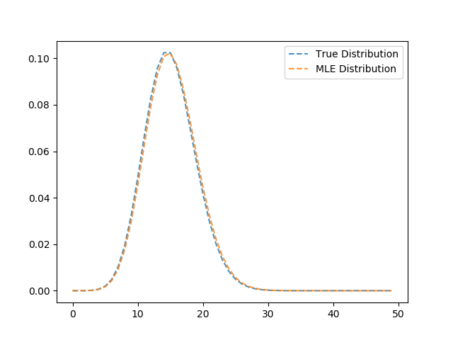
This code generates a sample of 100 poisson random variables, each with \(\lambda = 15\). The mle, lam_hat yields an estimate of 15.22, which is fairly close. Let’s compare the distribution functions of the true distribution and our MLE distribution,
import matplotlib.pyplot as plt
import math

def poiss(lam, k):
	return (np.exp(-1*lam)*(lam**k)) / np.math.factorial(k)

mle_pdf = np.zeros(50)
true_pdf = np.zeros(50)
for k in range(50):
	true_pdf[k] = poiss(lam, k)
	mle_pdf[k] = poiss(lam_hat, k)

plt.plot(range(50), true_pdf, ls='--', label='True Distribution', alpha=.8)
plt.plot(range(50), mle_pdf,  ls='--', label='MLE Distribution', alpha=.8)
plt.legend()
plt.show()
